Description
How to Use this Manual
This manual includes eight chapters covering the key tasks in doing your own forest inventory. The chapters follow a sequence, with each chapter building on the concepts covered in the preceding chapters. For this reason, we recommend that you work through the chapters in order. Chapters 5 and 8 are optional chapters for those who wish to go deeper into some more advanced inventory techniques.
Each chapter includes a list of recommended materials to complete the described tasks. More information about the materials referenced in this manual is provided in the next section. Each chapter will include “on your own” exercises to guide you in applying what you’ve learned to your own property. These exercises provide a step-by-step roadmap to successfully complete your inventory project. Some chapters also include links to online streaming videos to supplement the explanations in the text and give you a better feel for how to carry out various steps in the inventory process. A highspeed Internet connection is recommended for viewing these videos.
References and suggested further reading are included throughout the manual. Please refer to the glossary for unfamiliar terms used in this manual. The appendices contain additional materials, including data sheets to use when doing your inventory.
We strongly encourage you to enlist the help of your local Extension or state service forester, who can provide you with site-specific tips for applying the concepts in this manual to your property based on your ownership objectives. We also encourage you to work through this manual together with friends, family, and/or neighbors.
If you are part of a local landowner group, you may wish to work with other members and learn from each other.
Go further with the Landscape Management System (LMS) software
This manual is designed to help you gather inventory data that is compatible for use with a free (public domain) software program known as the Landscape Management System (LMS). LMS is a unique and innovative program that allows you to work with your inventory data to generate statistics about your forest, create representative images of your forest, predict how your forest will grow and change over time, and even experiment with different management alternatives. For instance, you will be able to model the effects of different types of thinning right after treatment, as well as 5, 10, or 20 years in the future or beyond. You will be able to assess outcomes relative to volume, revenue, wildlife habitat, fire risk, carbon sequestration, and more. Outputs include tables, charts, and realistic images of your forest, giving you powerful communication tools to share your objectives and outcomes with family members, co-owners, or other stakeholders. LMS allows you to examine the possibilities without putting your forest at risk—if you do not like an outcome, you can “put the trees back on the stump” and explore other alternatives. LMS is available for free download.
Materials Needed
Conducting a forest inventory does not require a huge investment in tools. Basic steps can be completed with little more than a measuring tape, compass, and a woodland stick, all of which are relatively inexpensive. For better results, however, you should plan to invest in tools such as a logger tape and a clinometer. These tools are more expensive, but they will yield greater accuracy and versatility, and they should last for many years. The most expensive tool on the list below will likely be the increment borer, but this tool is optional. Your local Extension or state service forester may have some of these tools available to borrow at little or no cost. WSU Extension publication EM038E1 also provides techniques for making your own forest inventory tools.
Minimum Requirements
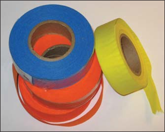
Colored ribbon
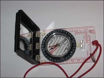
Hand Compass
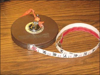
Measuring Tape
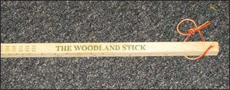
Woodland Stick
a yardstick and will allow you to measure tree heights and diameters quickly and easily. You can also use a diameter tape and clinometer instead of a woodland stick to perform these functions with greater accuracy (see Recommended tools below). Woodland sticks may be available for purchase for a nominal fee from your local Extension Forester.
Miscellaneous supplies
¹ Hanley, D. and J.A. Wagar. 2011. Simple Homemade Forestry Tools for Resource Inventories (pdf). WSU Extension publication EM038E.
Recommended tools
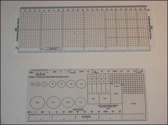
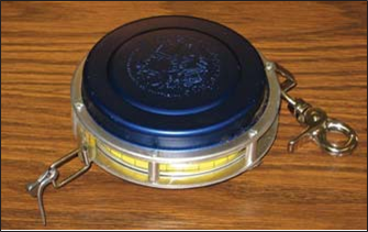
Acreage measuring grid
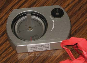
Clinometer
Diameter tape
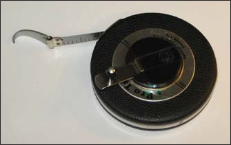
Logger tape
Calculator
Optional tools
Graph/grid paper
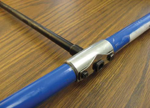
Increment borer
Orange timber marking crayon
Permanent marker
Prism
Keyhole angle gauge
Rope
Staff or stakes
Where to buy
The tools above are available from local logging or civil engineering supply stores as well as online forestry supply retailers. Below is a list (not exhaustive and with no implied endorsement) of several online retailers:
- Bailey’s – 1-800-322-4539
- Ben Meadows – 1-800-241-6401
- Forestry Suppliers – 1-800-647-5368
- Pac-Forest Supply – 1-877-736-5995
Chapter 1: Mapping your Forest
The first step in conducting a forest inventory is to get the “big picture” of your forest. Obtaining a good aerial image helps lay the foundation for your inventory. The image will help you to delineate forest stands and other important features.
Learning Objectives
- Obtain an aerial image of your property.
- Divide your forest into individual stands.
- Determine the area of each stand.
Materials Needed
- Computer with Internet access and a printer (if you do not own a computer, try the ones avail-able at your local library)
- Pencils and/or pens in several different colors
- Ruler
- Calculator (recommended)
- Acreage measuring grid (recommended)
- (SBQI/HSJE QBQFS (PQUJPOBM)
A. Create a basic map of your forest
The best way to get the big picture of your forest is to start with an aerial image of your property. Below are several potential sources of aerial images. Your local Extension or state service forester may be able to assist you in choosing an appropriate image source to use for planning your inventory.
- One of the best sources for aerial images may be your local county government. Many counties have images available online for free download and printing through the assessor’s office, plan-ning department, or similar department. Contact your local county government for information on availability.
- Your state department of forestry or natural resources (or equivalent department) may have aerial photography available. Contact the relevant department for your state for information on availability.
- Several Internet mapping sites can provide you with aerial images of your property that you can download and print for free. Coverage is limited in many rural areas, though. Here are some com-monly used websites:
- Google Maps you the option of searching for an address and viewing satellite imagery.
- Google Earth is a free tool you can download that can show you printable images of a given address/location.
- Microsoft Bing Maps is similar to Google Maps, allowing you to search for an address and view/print an aerial image.
- Terra Server is an-other free site that you can use to search for your location and see what aerial images are available.
- Forest*A*Syst is a free, interactive website for small forest owners that includes a tool for printing aerial photos of your property.
- The USDA-Natural Resource Conservation Service’s (NRCS) Web Soil Survey is primarily designed to provide soil maps of your prop-erty, but it also offers aerial image overlays. Having the soil map in addition will yield further benefits as you conduct your inventory, so this free site is worth exploring.
Whatever the source, a key to successfully working with an aerial image is that the scale, which is the ratio of distance on the image to actual distance on the ground (e.g., 1” = 300’), must be large enough to allow you to distinguish geographic features (roads and ponds, etc.), texture, and color in your forest.
B. Identify stands
To figure out where different stands are in your forest, it is important to look at aerial images as well as walk-ing your forest to examine it at the ground level. Start at a known location within your forest, such as near the house or a pond, or at the property line or corner. Look for areas on the ground with similar tree species composition, similar tree ages, etc. What areas of the forest look the same, and what areas look different? Correspond these areas to different colors, shades, and textures on the aerial image to get a bird’s eye layout of the stands on your property. If you have a map show-ing different underlying soil types on your property (see Chapter 8), this may further assist you in delineating stands. Your local Extension or state service forester may also be able to provide assistance with delineating stand boundaries.
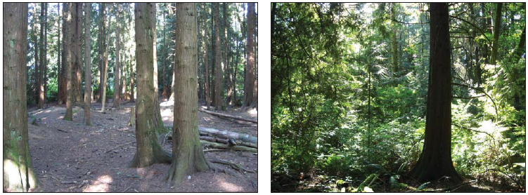
Figure 1-1 illustrates two areas that showed significant differences in color and texture on an aerial photo. An on-the-ground visit confirmed that the vegetation in these two areas was very different—one area had dense, coniferous vegetation with no understory, while the other was a mixed species stand with a diverse under-story. These areas would likely be managed differently, so they were identified as two stands.
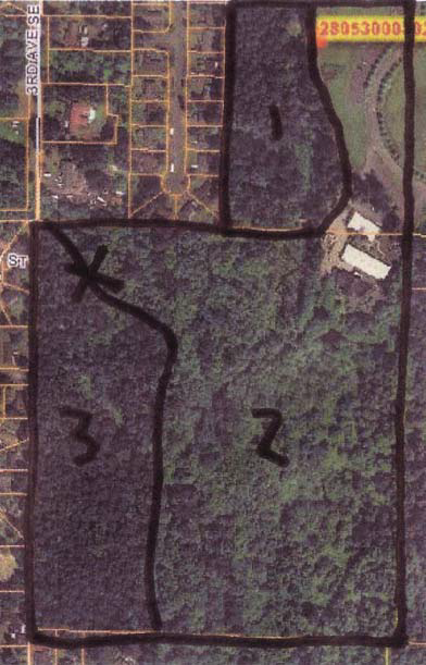
Figure 1-2 shows the end result once stands have been identified. Stand boundaries have been drawn on the aerial photo, which can now serve as a stand map.
Notice the difference in both color and texture between the different stands. Stand 3 is the dense, pure conifer stand shown on the left in Figure 1-1, whereas Stand 2 is the more diverse, mixed stand shown on the right in Figure 1-1. The “X” marked in the upper left denotes the location of the video clip above.
Once you have identified your stands, give each one a name or number to reference it. Some people simply number their stands. Others give descriptive names, such as “2006 Douglas-fir plantation” or “Mature Ponderosa pine stand.” Others may name a stand after a specific feature or something of personal significance, such as “Billy’s hillside stand” or “family picnic area stand.” It is possible that your property incorporates only one stand, especially if your property is small. Large properties may have many different stands.
On your own
Look at the aerial image that you created in the previous activity. See if you can identify potential stand boundaries. Walk your forest to help confirm their location. Draw the stand boundaries on your map and give each stand a name of your choosing.
C. Determine the acreage of each stand in your forest2
It will be helpful to estimate the acreage of the stands in your forest. This does not need to be exact—a reasonable estimate should work fine for our purposes (there are, however, applications such as a timber sale in which precise measurements of acreage, such as those done by a professional forester or surveyor, will be required).
You may be able to estimate acreage visually just by looking at your map. For example, if your property is 10 acres and you have two stands that each comprise approximately half of the property, you would estimate each stand to be 5 acres. Similarly, if you know the acreage of a given stand (for instance, one that was recently harvested), you could visually estimate the acreage for the other stands. This is the easiest but least precise way to determine acreage.
Another approach is to use an acreage measuring grid or area scale. This is a grid or series of evenly spaced dots, often printed on clear plastic. These grids are available from forestry supply merchants. You can also make your own using a piece of graph/grid paper and a clear plastic sheet.
Professional acreage grids usually have a key relating the grid squares or dots to acreage given a certain scale of map/photo. If your map/photo fits the pre-defined scale(s) on the acreage grid, you can overlay the grid on your map/photo, count the squares or dots that cover each stand, and use the key to calculate acreage.
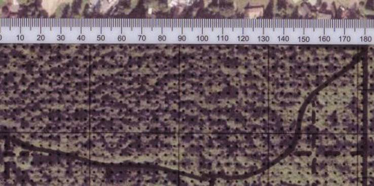
In many cases your map/photo will not fit the defined scale of the acreage grid. To resolve this problem, calculate how much area the dots or squares on the grid represent given your particular map/photo scale. Figure 1-3 shows an acreage grid with dots overlaid on an aerial photo of a stand. According to the acreage grid, each dot represents 1/10th (0.1) acre if the photo scale is 1” = 660’. However, the scale of this particular aerial photo is 1” = 300’, so a calculation is needed.
Below is how to set up the calculation. Note that the photo scales are squared to convert from units of length to area.
[Actual photo scale (feet per inch)]² x [Per dot acreage of grid] / [Assumed photo scale on grid (feet per inch)]²
Using the example in Figure 1-3, the actual photo scale is 300 feet, the per dot acreage of the grid is 0.1, and the assumed photo scale of the grid is 660 feet.
300² x 0.1 / 660² = 0.02, or 1/50th acre
Now that the grid has been converted to the photo scale, the next step is to count the dots that fall within the drawn boundaries of the stand. There are approximately 477 dots within the stand boundary in Figure 1-3; these dots multiplied by 0.02 acres per dot yield approximately 9.5 acres.
Another way to use the acreage grid is to simply determine how many dots or squares cover your entire property. For instance, if 100 dots cover your property, which you know to be 20 acres in size, that means there are 5 dots per acre and each dot represents 1/5 or 0.2 acres. Using this method avoids converting between the grid and photo scales.
On your own
Using your map with the stand boundaries drawn in, estimate the area of each stand using one of the procedures described above. Make a record of the acreage of each of your stands.
² In addition to the procedures described here, it is also possible to measure acreages by walking the boundaries of the unit with a GPS receiver. Many newer consumer-grade GPS receivers can estimate acreage within 1–2 tenths of an acre. The larger the acreage measured, the higher percentage accuracy. Using a GPS for this task also allows you to pull the path you took into a computer mapping program.
Chapter 2: Introduction to Plot Sampling
Chapter 1 focused on taking a “big picture” approach and dividing your forest into individual management units called stands. The next step is to inventory the trees in each stand. When conducting your forest inventory, we recommend working with each stand separately (also called stratified sampling). To inventory your trees, it would be unrealistic to measure every tree—even in a small stand. Instead, we do plot sampling. By measuring trees in small areas of your forest, called sample plots, you can then extrapolate the sampled information and get information about your forest as a whole.
Learning Objectives
- Establish a plan to systematically sample the stands in your forest.
- Determine how many plots you want to establish in each stand.
- Determine how far apart the plots should be in each stand.
- Identify on your map where the plots should be located.
Materials Needed
- The map you created in Chapter 1.
- Pencils and/or pens in several different colors.
- Ruler.
- Calculator (recommended).
A. Systematic Sampling
As stated in the introduction, it is impractical to count every tree in a stand, so you will be setting up sample plots and making determinations about the entire stand based on these small sample areas. When putting in sample plots, it is very important to be systematic. In other words, you want to have a pre-defined set of rules that will determine where sample plots are located. The purpose of a systematic sampling procedure is to avoid sample bias, which occurs when the samples taken are not representative of the stand.
Biased Example 1
Suppose you are trying to determine where to locate sample plots in your stand. You do not want to go deep into the stand because the terrain is steep and difficult to walk on, so you locate all of your plots along a road or trail. This would be a biased sample, because it only includes areas near a road or trail and does not represent the interior of the stand or areas away from forest edges.
Biased Example 2
Suppose you are trying to determine where to locate sample plots in your stand. You know of several key features that are important to you, such as a large, old oak tree or a special area along a stream that you like to visit. You decide to put your plots in these places so that you can be sure that these special features are included in your inventory. As with the example above, this is not systematic and will introduce bias into your inventory by over-representing things like large oak trees.
Biased Example 3
Suppose you are trying to determine where to locate sample plots in your stand. Parts of the stand are more open than others, allowing for easy access. You decide to locate your plots in these open areas to make it easier to navigate and measure the trees. Again, this is not a systematic approach and would introduce bias by over-representing the more open areas and under-representing the denser areas.
Biased samples result in an inventory that will not describe your forest accurately.
An easy way to set up a systematic sampling procedure is to overlay a grid on your stand map. Where the grid lines intersect on your map is where your plots should be located. This helps mitigate bias, as the plots fall based on the grid, not based on preferred or convenient locations. To fully minimize bias, there would also be a random element to the sampling, such as a random starting location or direction for the grid. For ease of implementation, the procedures described here do not include randomization. This may cause some level of bias in the sampling, but the overall results should still be adequate for the purposes of a stewardship planning inventory.
B. How Many Plots per Stand?
The question of how many plots per stand is not as straightforward as it might seem. The more plots you put in, the more accurate your inventory will be, but the more time and effort it will take to make the inventory. There are rules of thumb that can guide you, but ultimately it becomes a question of balancing the labor required with the accuracy desired.
In general, you should put in at least three total plots per stand. In smaller stands, this may mean that plots are close together. For best results, you should also strive to have, at a minimum, one plot for every 10 acres. For example, if you had a 50-acre stand, this would mean a minimum of five plots.
Consider the uniformity of the stand when determining how many plots to establish. If your stand is a young, uniform plantation, you might only need to measure the minimum number of plots. Conversely, for a very diverse stand of species, densities, and terrain, more plots may be needed for better representation. How many more you put in (and whether you even do the suggested minimum) ultimately depends on how much effort you are willing to invest. Just remember that with fewer plots your inventory will not be as accurate a representation, so treat the inventory data accordingly. Your local Extension or state service forester can assist you in determining an appropriate number of plots to meet your objectives.
On your own
Look at the stand map you created in Chapter 1. Note the acreage you determined for each stand. Also, consider how uniform or diverse each stand is. Based on this information, determine how many plots you wish to establish in each stand.
C. Determining how far apart plots should be
When setting up your plot grid, you will need to determine how far apart your grid lines should be on the ground. This will depend on the shape, size, and configuration of your stand.
When laying out your grid, it may be easiest to run the lines in the four cardinal directions (i.e., north–south lines and east–west lines). This way, assuming that your aerial photo and map are oriented with north at the top, your lines will then be parallel to the edges of the map or photo (and in-the-woods navigation will be simplest). However, it may be desirable to orientate the grid lines differently to accommodate the unique shape and orientation of your stand.
Choose an identifiable place on or near the border of the stand that you can easily find on the ground to be your starting reference point. This could be a property corner, bend in a road, road intersection, stream, or other identifiable feature. From this reference point, move a pre-determined distance into the stand (e.g., half of a grid width) to establish your first plot. Subsequent plots would then be located along a grid from there.
When establishing distances, a unit of measure that is often used in the forest is the chain, which is 66 feet. Both the distance from the edge to the first plot and the interval between plots will depend on the size of your stand. Table 2-1 suggests some distances.
Chains
The chain is a somewhat archaic unit of measure that was used for surveying in medieval times and is still often used today in agriculture and forestry. A chain is 66 feet long. There are 80 chains in a mile. An acre is 10 square chains, which corresponds to a rectangular area 1 chain by 10 chains (10 chains is also referred to as a furlong). If you have a 40-acre square property (i.e., a quarter-quarter section), your property would be 20 chains (or 2 furlongs) on each side.
D. Determining your plot locations
To draw distances in chains on your map and/or aerial image, you must determine how long these distances are on your map given the scale. You can use the following equation to determine a desired distance on the map:
[Map scale (inches) × desired distance (feet)] ÷ map scale (feet)
Map Scale Example
If your map scale is 1″ = 1,000′ and you want to know how long on the map 5 chains (5 × 66 = 330’) is, you would compute the following:
(1 × 330) ÷ 1,000 = approx. 0.3 inch
It is important to note the scale of your ruler. Most standard rulers are marked every 1/16th of an inch. If this is the case, you will need to know what a value such as 0.3 inch is in 16ths of inches. Table 2-2 gives approximate conversions from 10ths of inches to 16ths of inches. In this case we see that our example of 0.3 (3/10ths) inch = 5/16ths, so you would mark on your map 5-chain intervals every 5/16ths of an inch. This procedure can be done for any map scale or number of chains.
| Stand size | Distance from reference point to first plot | Grid interval distance |
|---|---|---|
| 2–5 acres | 1 chain (66 feet) | 2 chains (132 feet) |
| 5–10 acres | 1.5 chains (99 feet) | 3 chains (198 feet) |
| Over 10 acres | 2.5 chains (165 feet) | 5 chains (330 feet) |
Note that these distances are only suggestions. Depending on the shape and configuration of your stand and the location of your reference point, you may have to adjust these distances—but once your distances are determined, they must not be changed.
| 10ths | 16ths |
|---|---|
| 1 | 2 |
| 2 | 3 |
| 3 | 5 |
| 4 | 6 |
| 5 | 8 |
| 6 | 10 |
| 7 | 11 |
| 8 | 13 |
| 9 | 14 |
| 10 | 16 |
For larger stands, laying out your grid may result in more plots than you want or need to put in. For instance, if you have a 60-acre stand, a 5-chain grid should yield somewhere in the neighborhood of 24 plots. If it is a uniform stand, you may wish to do the recommended minimum of 6 plots (1 per 10 acres) or you may wish to do 10, 12, 15, or some other number of plots less than the 24 on your grid. The simplest way to reduce the number of plots is to widen your grid. For example, using a 10-chain grid instead of a 5-chain grid reduces the approximate number of plots from 24 to 9 in a 60-acre stand.
Example Plot Grid
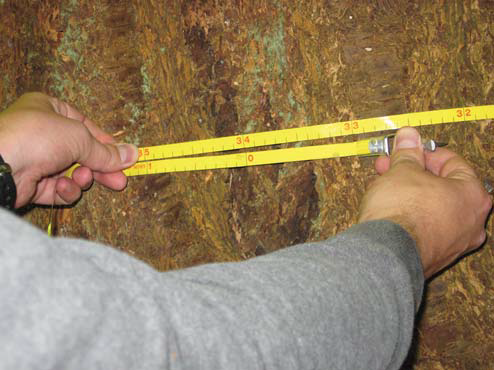
If you are laying out a plot grid in a stand that is approximately 23 acres, a minimum of 3 plots would be desired for good results. The recommended distance would be 2.5 chains from the reference point for the first plot and 5 chains between plots (Table 2-1). Holding a ruler up to the scale bar on the aerial photo shows that 100 yards (300 feet) is approximately 15/16ths inches (Figure 2-1). Using the equation from above, the map distance for 5 chains can be calculated:
[15/16ths × 330] ÷ 300′ = approx. 1″
In this example, 5 chains on the ground just happens to be 1 inch on the photo (when rounded to the nearest 1/16th inch). In most cases it will not be an even measure like this.
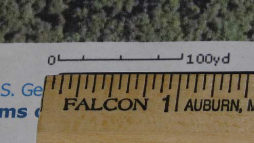
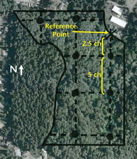
Figure 2-2 shows one possible plot grid. The reference point (marked with an “X”) is located at the corner of a building, which will be easy to find on the ground. Moving south 2.5 chains locates the first plot. Subsequent plots (marked as black dots) are established on a 5-chain grid. In this example, eight plot locations have been identified. Notice how they are systematically distributed through the stand.
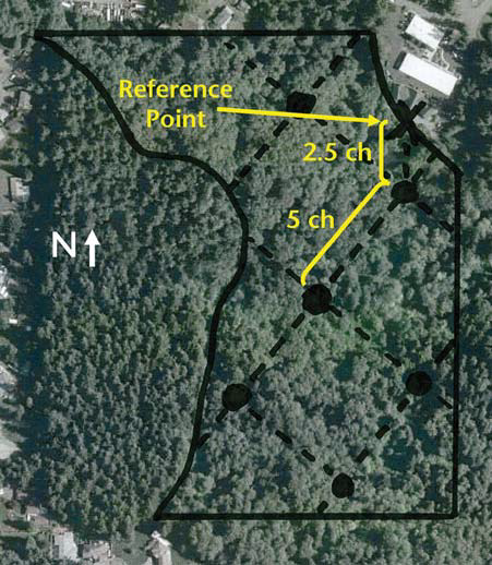
The grid orientation, starting point, or width can be adjusted to achieve the desired number and distribution of plots. For example, Figure 2-3 shows an alternative grid configuration. The reference point and first plot are located in the same place as Figure 2-2, but the grid lines run northwest to southeast and northeast to southwest. This results in a systematic distribution of six plots instead of eight.
On your own
Choose a stand on your property. From the previous on your own exercise, you should already know how many plots you wish to put in. Using the techniques described above, lay out a plot grid and mark the locations where your plots will be (and the interval distances and distances from reference points) on your map. It helps to have multiple copies of your map printed, as it often takes several attempts to draw a plot grid that works. Additional copies also allow you to make separate maps for different features (e.g., stands, roads, streams, etc.). You are now ready to go to the woods. A plastic slip cover will help protect your map(s) from the weather.
Chapter 3: Locating Plots on the Ground
So far, you have identified individual stands in the forest, learned about plot sampling, and marked locations on a map of where your inventory sample plots will go. Now it is time to head to the woods and locate on the ground the plots that you have marked on your map.
Learning Objectives
- Pace out distances in the woods.
- Set declination on a compass.
- Use a compass to navigate in the woods.
- Establish a plot center.
Materials Needed
- Measuring tape
- Compass
- Your map
- Colored ribbon
- Stakes or staff (optional)
A. Pacing
In Chapter 2, you established plot locations on a map with pre-determined distances (measured in chains) between plots and from a starting reference point. When locating these plots on the ground, you will need to measure out these distances. It can be onerous and time-consuming to use a measuring tape to measure out the distances in the woods. It is quicker and easier to pace out the distances.
Pacing is simply counting your steps. If you know how many steps (paces) it takes to travel one chain, you can count this out as you walk to estimate the distance. This estimation is not as accurate as actually measuring the distance, but it can be surprisingly close. More importantly, it is still part of a systematic way to locate inventory plots and any minor discrepancies between paced and actual distances should not introduce bias to the sample.
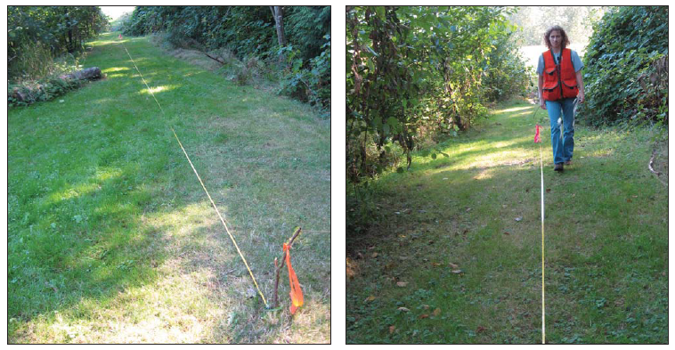
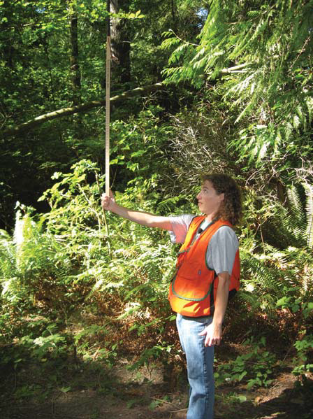
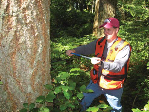
The first step in pacing is to figure out how many paces it takes you to walk one chain. To do this, find a flat, open area (a lawn or driveway works well) and use a measuring tape to mark out a course of one chain (66 feet). Walk the course several times, counting your paces as you go (Figure 3-1). When counting paces, it may be easier to count every other step (i.e., one complete stride). In other words, if you lead with your left foot, count every time your right foot hits the ground. Try to walk as naturally as possible—do not take extra-small or extra-large strides. As you walk the course multiple times, you may get slightly different counts, so use an average of these counts.
B. Setting declination on a compass
Not only do you need to go the appropriate distance in the woods, you also need to travel in the right direction. Recall from Chapter 2 that for each stand you established grid lines, originating at an identifiable reference point on the ground. You will need to use a compass to guide you in the direction of your grid line to find your plot.
When using a compass, it is important to set the declination for your location. Declination adjusts the compass for the difference between true or geographic north (i.e., the North Pole) and magnetic north, where the compass needle points, which is somewhere in the Canadian Arctic but shifts every year. (For more information on declination)
NOAA has an online tool to compute declination for your area. With this tool, you can enter your zip code to determine latitude and longitude, and then compute the declination, which will yield both a number (in degrees) and a direction (either east or west).
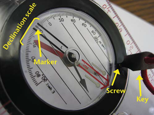
Once you know the declination value for your area, you can set this on your compass (assuming that your compass is adjustable for declination—some less expensive compasses may not be). This usually involves turning a small screw with a “key” provided with your compass. Consult the instructions provided with your compass to determine exactly how declination is adjusted with your specific model. As you set declination, be mindful that it can be east or west, so be sure to set it in the correct direction (Figure 3-2).
Once declination is set, your compass will now automatically account for the differences between true north and magnetic north and your compass will point to true directions based on your specific location. Because magnetic north continues to shift over time, you should check and update the declination of your compass every few years.
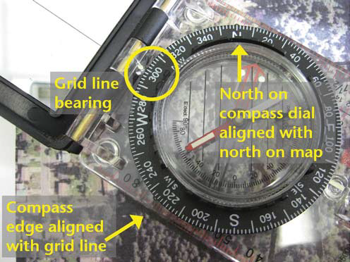
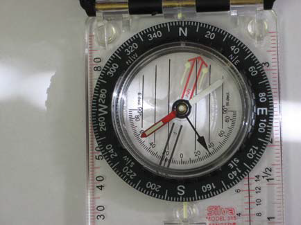
on the map, and the resulting compass reading is the direction of travel for the grid line, in this case 300º on an azimuth-style compass (see sidebar discussion of the difference between quadrant and azimuth compasses).
C. Find your direction of travel
Now that your compass is set for declination, you are ready to find your direction of travel on the ground. You should first determine whether north is on your photo/map. All commercially available aerial photographs have true north at the top. If you obtained your aerial map from an Internet source, be careful to note true north. Lay your compass on your map such that the edge of the compass lies along your grid line (pointed in the direction of travel). Turn the compass dial so that north on the compass dial is pointing towards north on your photo/map. The compass reading will give you the direction of travel for your grid line (Figure 3-3).
Once you have the direction of travel to your first plot, go to the starting reference point. Rotate the dial on the compass to set the direction you want to go. Now, holding the compass level, turn the whole compass until the needle lines up with the arrows. Your compass is now pointing the direction you want to go. As you travel, you will need to hold the compass level in front of you and keep the compass oriented such that the needle stays lined up with the arrows. If your compass has a mirror, you can tilt the mirror down to allow you to see the orientation of the needle while sighting through a notch at the top to sight your course ahead (Figure 3-5).
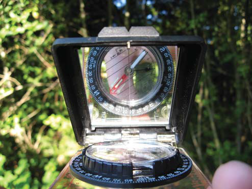
level. Sight through the notch at the top to see where you need to go.
A helpful technique is to sight ahead and identify a feature that is along your travel direction (e.g., a tree). Walk towards this feature and, when you arrive, sight ahead to the next identifiable feature along your travel direction. Continue this until you have gone the correct distance (remember to count your paces). It is often useful to leave a small piece of survey ribbon at the point you started so that you can return to that place easily in the event that you forgot how many paces you went (or to retrieve that piece of equipment that was left behind).
Note that, depending on your brand and style of compass, the technique may be slightly different than what is shown here. Please be sure to read the operating instructions that came with your compass so that you know how to correctly operate it.
Quadrants vs. Azimuth
There are two styles of compass: quadrant and azimuth. A quadrant compass (Figure 3-4a) is divided into 4 quadrants, each reading from 0° (starting with north or south) to 90° (ending at east or west). An azimuth compass (Figure 3-4b) reads from 0° (north) all the way around the compass to 360° (back to north).
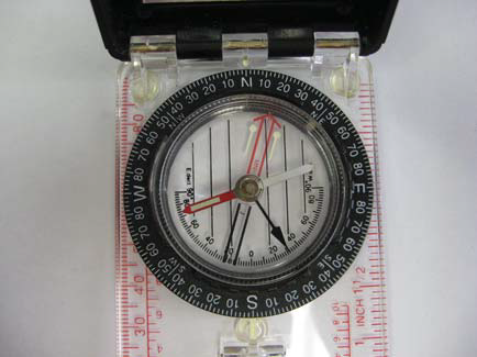
If you want to travel northeast, on a quadrant compass this would be expressed as N 45° E (45° east of north). On an azimuth compass it would be expressed as 45°. Similarly, if you wanted to travel southwest, this would be expressed on a quadrant compass as S 45° W (45° west of south) compared to 225° on an azimuth compass. Make sure to note which type of compass you have and consult the operating instructions for your compass for more information.
Chapter 4: Establishing Fixed-Radius Plots
In previous chapters, you mapped out your stands, identified where sample plots will go, and learned how to navigate in the woods to your first plot location. This chapter will teach you how to establish a fixed area plot. Advanced users may also wish to read Chapter 5 to learn about a variable area plot. As a reminder, you are sampling your stand using plots so that you can extrapolate the data collected to the full stand on a per-acre basis.
Establishing plots and collecting data in them is much more manageable when you are working with a partner. Dividing the labor makes things go faster; for example, one person can be standing at the center of the plot and recording data while the other delineates the plot or takes tree measurements.
Learning Objectives
- Determine an appropriate plot size.
- Establish the boundary of a fixed plot.
- Identify and count “in” trees (sample trees).
- Understand the relationship between the number of trees in a plot and the number of trees in a stand on a per acre basis.
Materials Needed
- Measuring tape or logger’s tape
- Colored survey ribbon
- Orange timber marking crayon (optional)
- Permanent marker (optional)
- Rope (optional)
A. Plot size
Just as it sounds, a fixed area plot has a known area. When you establish the first plot in any given stand, you will need to choose an appropriate plot size. This size should then be used throughout the rest of the stand. You will want to choose a plot size that gives you an average of 5 to 10 trees per plot. Try a starting plot size such as 1/20th of an acre, and see if you get in the neighborhood of 5 to 10 trees.
If you find that the trees in your stand are widely spaced such that you have very few trees in your plot (4 or fewer) and this wide spacing looks to be consistent throughout the stand, consider increasing your plot size (e.g., to 1/10 acre). Similarly, if your stand is dense such that you have numerous trees (12 or more), consider smaller plots (e.g., 1/30 acre).
B. Establish the boundary of your fixed plot
Plots can be established in various shapes, but circular plots are the easiest to use in a forest. To establish your circular plot, you will need to know the plot radius, which is the distance from the plot center to the outer edge of the plot (Figure 4-1). Table 4-1 shows plot radius values for a range of plot sizes.
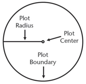
Figure 4-1: The plot radius is the distance between the plot center and outer boundary of the plot. Table 4-1 lists plot radii for different-sized plots.
To establish your plot boundary (i.e., perimeter), start at plot center and walk out the prescribed distance in various directions and hang a colored survey ribbon on a nearby branch or shrub to mark the plot boundary. You should go out at least six different directions to get a good sense of where the plot boundary is. Once you have six or more flagged points marked around your plot boundary, you will need to visually “connect the dots” to estimate the complete boundary of your plot.
When measuring out the distance from your plot center to your plot boundary, you can use a cloth measuring tape or a logger’s tape. You can also use a rope that has been pre-cut to the length of your plot radius. This may save time and effort in marking your plot boundary.
circular plots.
| Plot Size (acres) | Radius (feet) |
|---|---|
| 1/5 | 52.7 (≈52’8”) |
| 1/10 | 37.2 (≈37’2”) |
| 1/20 | 26.3 (≈26’4”) |
| 1/30 | 21.5 (≈21’6”) |
| 1/40 | 18.6 (≈18’7”) |
| 1/50 | 16.7 (≈16’8”) |
| 1/60 | 15.2 (≈15’2”) |
| 1/100 | 11.8 (≈11’10”) |
| 1/250 | 7.4 (≈7’5”) |
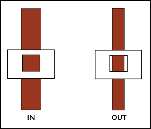
C. Determining “in” trees
Now that you have marked the boundary of your plot, you will need to determine which trees are in the plot. A tree is considered “in” if the center of the tree falls within the plot boundary. Starting from a given direction (e.g., north, or the direction you traveled to get to the plot), systematically work your way around the plot in a clockwise direction and identify your “in” trees. It may be helpful to flag these trees with colored survey ribbon as you go. You can use a permanent marker to number the flags to help you keep track of each tree. You can also use an orange timber-marking crayon to mark/number the “in” trees.
When identifying trees in your plot, there should be a minimum size limit. For the purposes of this manual, we will focus on overstory trees, which we will define as live trees that are at least four inches in diameter at breast height (DBH). (See Chapter 6 for more information about DBH.) Snags (dead trees), smaller trees, and other features of the stand may also be of interest to you, depending on your management objectives and the purposes of your inventory. There are techniques to inventory these features. See the sidebar for an example of how to use stocking plots to measure reforestation. Your local Extension forester may have additional examples and suggestions on how to include special features of interest in your inventory strategy.
You may run into the issue of borderline trees that appear to be on the plot boundary. If necessary, run the tape or rope from the plot center directly to the tree to determine whether the center of the tree at breast height falls inside or outside the plot boundary. Figure 4-2 shows a schematic of a fixed plot with “in” trees identified in blue.

along the plot boundary are determined as “in” or “out” based on whether the center of the tree falls within the plot.
D. How do plot trees relate to the larger stand?
An advantage of fixed area plots is that the relationship between a plot tree and the larger stand is straightforward. For example, a tree in a 1/20th acre plot would represent 20 trees per acre (TPA) in the larger stand. This is also referred to as the tree’s expansion factor. When multiple plots are established, the number of trees per acre computed for each plot are added together and divided by the number of plots to establish an average value.
Example
Suppose you put in three 1/20th acre plots in a stand and count 5, 7, and 8 trees, respectively, in each plot (Table 4-2). Each plot tree represents 1 × 20 = 200 trees per acre in the stand, for a computed value of 100, 140, and 160 trees per acre in each plot, respectively. Adding these numbers up and dividing by three (the number of plots) yields an average of approximately 133 trees per acre in the stand.
| Plot | Trees | TPA |
|---|---|---|
| 1 | 5 | 100 |
| 2 | 7 | 140 |
| 3 | 8 | 160 |
| Sum of plots | 400 | |
| Average of plots | 133 |
³ Green, D., M. Bondi, and W. Emmingham. 1997. Mapping and Managing Poorly Stocked Douglas-fir Stands (pdf). OSU Extension publication EC113.
Chapter 5: Establishing Variable Plots (for advanced users)
In Chapter 4, we talked about fixed area plots. Now we will talk about a different kind of plot, which is a variable plot.
Learning Objectives
- Understand how a variable plot works.
- Choose an appropriate prism factor.
- Use a prism or angle gauge to determine “in” trees.
- Understand what the trees in a plot represent in a larger stand.
Materials Needed
- Glass wedge prism(s) or keyhole angle gauge
- Colored survey ribbon
- Orange timber marking crayon (optional)
- Permanent marker (optional)
A. Variable plots
Unlike fixed plots, which have a defined area, variable plots do not have a specifically defined plot size. An angle gauge (tool described in the Materials Needed section) is used to determine whether a tree is “in” (included in the plot sample) or “out” (not included in the plot sample) rather than the tree’s location within a defined boundary. The larger a tree is or the closer it is to plot center, the greater the likelihood of it being an “in” tree. Many professional foresters use variable plots instead of fixed plots because variable plots are more efficient at sampling trees to estimate stand volume.
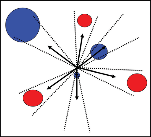
Conceptually, an angle gauge is used to determine which trees are “in.” Figure 5-1 shows a schematic of a variable plot in which an angle gauge is applied in several different directions. Trees intersected by the angle are “in” (shown in blue), while trees cleared by the angle are “out” (shown in red). Note how trees have to be larger to be considered “in” the further they are from plot center.
Variable plots are not as conceptually straightforward as fixed plots and require additional, specialized tools (prism or other angle gauge). However, the procedures for laying out a variable plot may be faster and easier than for a fixed plot, especially if you are working alone, on a steep slope, or with lots of brush.
B. Different prism factors
As with fixed plots, you want to have 5–10 trees per plot. To get the appropriate number of trees per plot, you will need to select a prism or other angle gauge with an appropriate basal area factor (BAF). If your stand has, on average, larger trees, you will want to use a larger BAF (e.g., a BAF of 40). If your stand has, on average, smaller trees, you will want to use a smaller BAF (e.g., a BAF of 10 or 20).
The most important purpose of the BAF when doing field measurements is to choose one that will give you the desired average number of trees per plot. Remember that each prism has a fixed BAF. Similar to fixed plots, once you have selected the BAF that you are going to use, you need to stick with it for each and every plot in the stand.
C. Using an angle gauge
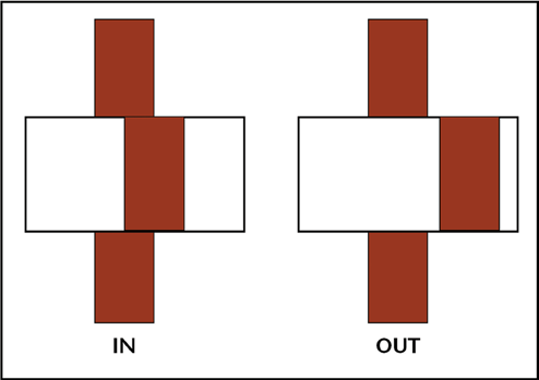
Two types of angle gauges are commonly used for variable plots. A glass wedge prism is a piece of glass that has been specially cut to deflect light and displace a tree’s image. They are calibrated and very precise. Holding the prism vertically⁴ over plot center, look at the trunks of the trees around you (at breast height) through the prism. The trunk of the tree as seen through the glass prism will be shifted. If the shifted image of the tree trunk overlaps what you see with your naked eye, the tree is “in.” If the shifted image of the tree trunk is completely separated from what you see with your naked eye, the tree is “out” (Figure 5-2). Make sure that as you work your way around the plot, you keep the prism fixed over plot center. You will see as you move around the plot that the further from plot center a tree is, the larger it must be to be considered “in.” The selection of “in” trees is thus a function of tree diameter and distance from the plot center.
Glass wedge prisms are delicate and expensive, and you may need several for different BAFs. A durable, inexpensive alternative that can replace several glass prisms (i.e., serve the same function) is a keyhole angle gauge, such as a Cruz-All. It has openings of various widths corresponding to commonly used BAFs.
Unlike the glass prism, with the angle gauge your eye should stay fixed over plot center rather than the device. The Cruz-All has an attached chain to help you keep it a prescribed distance from your eye as you look through it. Hold the end of the chain up to your face and hold out the Cruz-All so that the chain is taut. As you pivot around your plot center, look at trees through the opening that corresponds to your desired BAF. If the tree stem (at breast height, which is 4.5 feet above the ground) completely fills the opening, the tree is “in.” Otherwise, it is “out” (Figure 5-3).⁵
Basal Area Factor
Any tree that is determined to be an “in” tree represents the average amount of basal area in the stand. Basal area is the cross sectional area of the trunk of a tree at breast height (i.e., 4.5 feet above the ground). For instance, if you establish a variable plot using a BAF 40 prism, every “in” tree would represent 40 square feet of basal area regardless of the actual basal area of each tree. Thus if you had three trees in a BAF 40 plot, it would represent 120 (3 × 40) square feet of basal area per acre. The cumulative amount of basal area in a stand reflects both the size and density of the trees and is used commonly as a measure of whether or how much the stand should be thinned to meet a particular management objective.
Since basal area is directly related to a tree’s diameter, you can use mathematical formulas to take a tree’s diameter and the BAF used and compute that tree’s expansion factor (trees per acre). However, for our purposes now, determining figures such as basal area and trees per acre are not as important when taking field measurements. These calculations are covered later in Chapter 7.
As with fixed plots, you may occasionally run into a borderline tree. A common solution is to only count every other borderline tree as you inventory a stand.
On your own
Using a glass wedge or keyhole angle gauge, look at the trees around your plot center to get a quick count of the “in” trees. You may need to try a couple different BAFs to get the appropriate number of trees in your plot. Once you settle on a BAF, use it throughout the stand. Flag or mark all the trees that are in your plot (as described in Chapter 4). You are now ready to measure your plot trees (Chapter 6).
⁴ If you are looking up or down a significant slope at the tree, tilt the prism sideways (e.g., clockwise) to match the angle of the slope.
⁵ Steep slopes introduce errors that may require mathematical corrections when using keyhole angle gauges, so a glass prism may be an easier tool to use in these situations.
Chapter 6: Measuring Trees
In Chapters 4 and 5, you learned how to establish either a fixed plot or a variable plot. With your plot established and your “in” trees tallied, now it is time to measure the trees in the plot as representative samples of the trees in your stand.
Learning Objectives
- Measure a tree diameter at breast height (DBH).
- Measure a tree’s total height.
- Determine a tree’s live crown ratio.
- Determine a tree’s age.
Materials Needed
- Diameter tape or woodland stick
- Clinometer or woodland stick
- Increment borer (optional)
- Data recording sheets
A. Getting Started
You will need to record data about the trees in your plot. Several plot data sheets are included in Appendix C; you may photocopy these to make additional copies. You will need a sheet for each plot that you do. You can copy or print these sheets onto waterproof paper (available from forestry suppliers) to create durable, all-weather plot cards.⁶
On your plot data sheet, record the tree species for each tree in your plot. For some guidance on tree identification, see OSU Extension publication EC1450;⁷ WSU Extension publication EB0440;⁸ or UI publication *Wild Trees of Idaho.*⁹
B. Measuring tree diameter
After recording your tree species, the next step is to measure the diameter of each tree. Diameter is the width of a circle or cylinder, in this case the stem of the tree. Tree stems taper such that they are wider at the base and narrower further up. Thus, diameter will vary based on how high up on the stem of the tree you measure it.
A standardized height for measuring tree diameter is known as breast height, which is defined as 4.5 feet (54 inches) above the ground on the uphill side of the tree. Use a measuring tape to figure out how high up breast height is on you. Memorize this spot (e.g., the next to the top button on your shirt or coat¹⁰) so that as you stand next to a tree, you know where to measure diameter.
Using a diameter tape to measure DBH
The most accurate way to measure a tree’s diameter at breast height (DBH) is to use a special measuring tape known as a diameter tape. A diameter tape is calibrated such that circumference measurements are automatically converted to diameter (i.e., the measurement units have been divided by the constant Pi [equal to approximately 3.14 and represented by the Greek letter π]). Thus when you are physically measuring the circumference of the tree, you are reading the measurement in diameter units.¹¹ If you do not have a diameter tape, you can use a regular cloth measuring tape and divide your circumference measurement by Pi to convert to diameter.
To measure DBH, wrap the diameter tape around the tree at breast height, making sure the tape is level and not twisted. Most diameter tapes will give you diameter to the nearest 1/10th inch. Read the diameter measurement where the tape overlaps with the zero marker (Figure 6-1). If the tree is large, it is helpful to work with a partner to wrap the tape around the tree. Many diameter tapes also have a nail or hook on the end that you can stick into the tree to hold the end of the tape in place while you wrap it around. If the tree is markedly leaning, measure at an angle perpendicular to the axis of the tree to ensure that you are measuring the minimum diameter around the stem. If the tree is forked, measure it as one or two trees based on whether the fork is above breast height (one tree) or below (two trees).
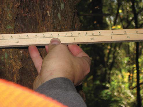
Using a woodland stick to measure DBH
A second way to measure DBH is to use a woodland stick (also called a Biltmore stick or a cruiser stick).
These special measuring sticks are inexpensive compared to diameter tapes and they are quick and easy to
use, but not as accurate as a diameter tape.
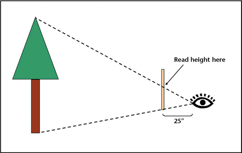
To use a woodland stick, find the side of the stick that is marked for tree diameter. With this side facing you, hold the stick up against the tree at breast height. The stick should be 25 inches away from your eye, which is a comfortable arm’s reach for an average person. Keeping the stick level and perpendicular to your line of sight, visually line up the left side of the stick with the left edge of the tree. Now, keeping your head still, move your eyes to the right edge of the tree and read where it falls on the stick (Figure 6-2). Note that woodland sticks usually only measure to the nearest inch (not as precise as the diameter tape). Since trees are not perfect cylinders, you should measure two perpendicular sides of the tree and average the values together to estimate DBH (Figure 6-3).
Quick Steps for Measuring DBH with a Woodland Stick
- Hold the stick against the tree at breast height, 25 inches from your eye.
- Visually line up the left edge of the stick with the left edge of the tree.
- Moving your eyes (not your head!), read where the right edge of the tree falls on the stick.
- Repeat the measurement for a different side of the tree and take the average.
C. Measuring tree height
After recording each tree’s diameter, measure their heights. Depending on how you intend to use your inventory data, you may not need to measure the height of every tree in the plot. For calculating the average height of the trees in your stand or for calculating volume per acre using the Tarif system (see Chapter 7), a general rule of thumb for an even-aged stand is to measure a minimum of six trees for each species in the stand, distributed across your plots. However, if you plan to calculate volume per acre using a standard volume table, you may need to measure the height of every plot tree.
If you wish to compute the site index (see Chapter 8), you will also need to include height measurements for several dominant, undamaged trees. Your site index trees can be the same trees you are already measuring height for, as long as they are dominant and undamaged. Approximately six trees total, well-distributed across the stand, should be measured per species for site index purposes.
As with other aspects of inventory sampling, it is desirable to be systematic when selecting a tree to take a height measurement (if you are not measuring every tree height). One method is to start from either north or whatever direction you were traveling to reach your plot, go clockwise around your plot, and select the first “in” tree of each species represented in the plot.
Using a clinometer to measure tree height
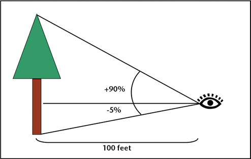
As with DBH, we will talk about two different ways to measure height. The first way is to use a tool called a clinometer. A clinometer is a vertical angle gauge that measures the slope from your eye to either the top or bottom of the tree. Looking with one eye into the hole of the clinometer, you will see a graduated scale showing the slope measurements. The scale will move up or down as the clinometer is tilted up or down. Different clinometers measure slopes in different units, so it is important to consult the instructions for your clinometer to confirm what units are being measured. Commonly clinometers list the slope in degrees on the left half of the scale and in percent on the right half of the scale.¹² The steps described below correspond to percent slope measurements. By definition, percent slope is the distance up or down per 100 feet of horizontal distance. Thus, a reading of 30% means a height or depression of 30 feet when measured at 100 feet horizontal distance.
When measuring the height of a tree, you will need to move away from the tree to a place where you can see the top. While you can choose any distance at which you can see the top of the tree and the clinometer reading is out of the top scale (usually 150%), though accuracy may deteriorate beyond 120% or so), because you are working in percent, a distance of exactly 100 feet will greatly simplify the calculation to determine tree height. For trees that are tall enough such that 100 feet is not far enough back to accommodate the scale of the clinometer (or to see the top of the tree), you will have to move back further to obtain an accurate reading. For very short trees, you may only need to move back 50 or 75 feet.
You can measure your distance away from the tree using a cloth measuring tape or a retractable logger’s tape. When choosing a spot from which to measure a tree, if you are on a slope, try to stay on the same level as the tree. If you go significantly uphill or downhill from the tree, your distance measurement (and subsequent height measurement) will not be accurate.
Once you have measured the distance from the tree, you can use the clinometer to measure the slope between your eye and both the top and bottom of the tree (Figure 6-4). Looking into the clinometer with one eye (you cannot actually look through the clinometer) and sighting the top of the tree with your other eye, visually line up the horizontal marker in the clinometer with the top of the tree (Figure 6-5). It may take some practice to get your eyes to work together for this. Once the horizontal marker in the clinometer is lined up, read the corresponding value on the percent scale. Now repeat this procedure for the bottom of the tree.¹³
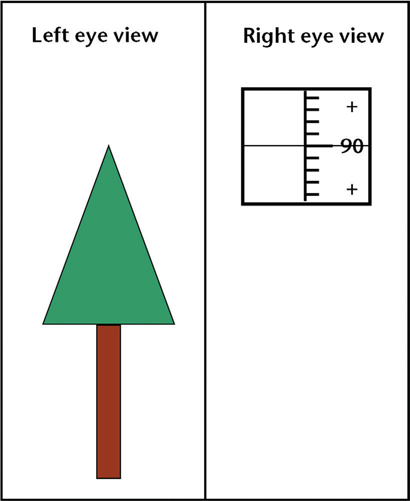
horizontal marker in the clinometer with the top of the tree and read the value (in this case, 90%).
Quick Steps for Measuring Tree Height with a Clinometer
- Move back a measured distance from the tree, preferably 100 feet.
- Looking at the top of the tree with one eye and through the clinometer with the other, line up the horizontal marker in the clinometer with the top of the tree, and read the value on the percent scale.
- Repeat this for the bottom of the tree. If the percentage to the bottom is on the negative part of the scale, add it to the percentage from Step 2; if it is positive, subtract it.
- Multiply the combined percentage by the distance back from the tree to determine the total tree height.
Example
- Distance from tree = 100’
- Tree top reading = +90%
- Tree bottom reading = -5%
- Combined reading = 90% + 5% = 95%
- Tree height = 95% × 100’ = 95’
Assuming the angle to the top of the tree reads a positive value, if the angle to the bottom of the tree reads a negative value, add the bottom value to the top value to get the total percent slope. In the case where the angle to the bottom of the tree also reads a positive value, such as when you are standing downhill from the tree (Figure 6-6), subtract the bottom value from the top value to get the total percent slope.
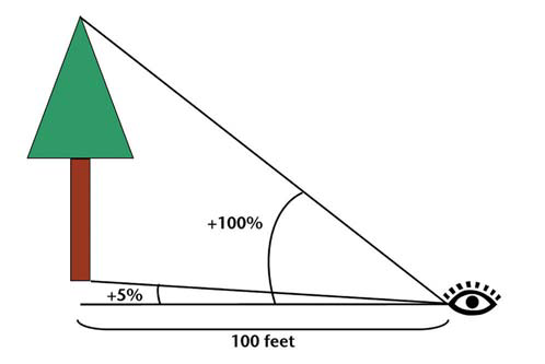
Try to measure tree height from roughly the same ground level as the tree. If the tree is on a slope, moving sideways away from the tree to take the measurement rather than up or down slope will help you remain level. If you move significantly up or down slope from the tree, your horizontal distance will need to be adjusted to account for the slope in order to measure the height accurately.
The total percent slope is equal to the vertical distance (i.e., the total height of the tree from top to bottom) divided by the horizontal distance away from the tree. Since we know the horizontal distance and the total percent slope, we can solve for tree height by multiplying the percent slope (expressed as a decimal) by the horizontal distance (Figures 6-5 and 6-6). This is why being exactly 100 feet away makes for the simplest calculation—a total slope of 95% means the tree is 95 feet tall (e.g., Figure 6-5). When using horizontal distances other than 100 feet, it may be helpful to have a hand calculator to assist with the calculation.
Using a woodland stick to measure tree height
You can also measure tree height using a woodland stick. This is an inexpensive option if you do not have a clinometer, though it is not as accurate. Similar to using a clinometer, you will need to use a cloth tape or logger tape to measure back from the tree a specified distance. With the woodland stick, this is a fixed, prescribed distance, usually 66 feet or 100 feet depending on your region and the stick you are using. Find the side of the woodland stick that is marked for tree height, and with this side facing you, hold the stick vertical. The stick should be 25 inches away from your eye. Keeping the stick straight, visually line up the bottom of the stick with the bottom of the tree (Figure 6-7). Now, keeping your head still, move your eyes to the top of the tree and read where it falls on the stick (Figure 6-8).
D. Determine live crown ratio
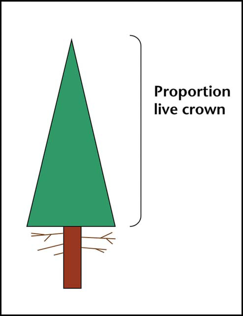
The live crown ratio is the proportion of a tree’s height (Figure 6-9). This provides information about the health of your trees and whether they are spaced adequately. If the live crown ratios are too low, the trees are weakening and may need to be thinned to provide more crown space. Crown ratio can be determined with a simple visual estimate. The live crown ratio should be estimated for each tree in the plot.
Quick Steps for Measuring Tree Height with a Woodland Stick
- Stand the prescribed distance away from the tree (usually 66’ or 100’ depending on the woodland stick).
- Hold the stick vertically, 25 inches from your eye.
- Visually line up the bottom edge of the stick with the bottom of the tree.
- Moving your eyes (not your head!), read where the top of the tree falls on the stick.
E. Determine tree age (optional)
While tree age is not a required part of forest inventory, it may be useful to gather this information if you do not know the age of your stand. You can determine the age of a stand by taking the ages of several dominant trees from different plots and computing the average of these values. If you have selected trees to measure for computing a site index, you will need to take the ages of those trees as well as their heights. See Chapter 8 for more information on computing a site index.
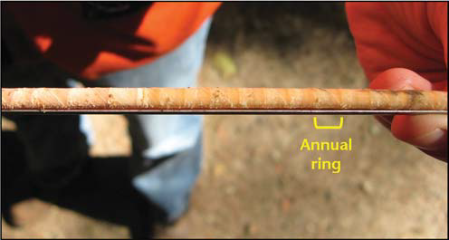
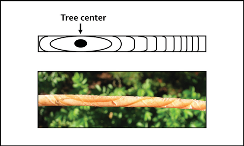
To determine the age of a tree, you will need a special tool called an increment borer. An increment borer is a hollow drill that allows you to extract a thin segment of wood called an increment core from the stem of the tree. The increment core will show the annual rings (Figure 6-10), which can be counted to determine tree age.
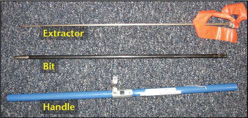
An increment borer has three parts: the handle, the bit, and the extractor (Figure 6-11). To assemble an increment borer, fir the back end of the bit into a notch in the center of the handle and clip into place (Figure 6-12). The extractor should be kept separate while boring. The extractor is easily bent, so handle it carefully and place it someplace safe while you are boring so that it does not get stepped on or damaged (in the hands of a trusted partner is ideal). You may also want to tie a piece of bright-colored ribbon onto the extractor to make it easier to find in the event it is dropped in heavy brush.
To use an increment borer, begin drilling into the tree at breast height by turning the handle clockwise. Make sure to keep the increment borer level and the drill straight in toward the center of the tree (Figure 6-13). You may need to apply pressure towards the tree when first starting until the bit catches on the wood (i.e., push and turn at the same time). You may hear creaking or popping sounds as you drill into the tree. Be sure to drill in far enough to reach just past the center of the tree.
Once you have drilled far enough to reach the center of the tree, carefully insert the extractor into the bit (spoon side up). You will feel some resistance. Once the extractor is all the way in, back the bit out one full turn (counterclockwise).¹⁴ Now slowly pull the extractor out; the increment core should come with it. If the core does not come out on the first try, reinsert the extractor and try again.
Once you have extracted the increment core, set it and the extractor aside. Be careful with the increment core,
as it is delicate and may fall apart easily. You should immediately begin removing the bit from the tree by turning the handle counterclockwise, as the increment borer may become stuck if left in the tree too long.
Once the increment borer has been removed from the tree, you can return to your increment core and begin
counting rings. If you successfully reached the center of the tree, you should see a round or oval-shaped ring on the increment core that marks the center (Figure 6-14). Begin counting with this center ring and count outward to the end of the increment core. Note that you are measuring breast height age, which is typically the value of interest. If you also want to know the total age, adding 4-5 years to the breast height age will in most cases give you a reasonable approximation.
When you have finished counting the rings, you may save or discard the increment core. Inserting the core back into the tree is not recommended, as this may introduce pathogens into the stem of the tree.
It is important to take care of your increment borer so that it will last for many uses. Make sure to always protect the sharp end of the bit from getting chipped or dented. Do not let it come in contact with metal or rock. It is important to check the bit after each use to make sure it is clear of any leftover wood fragments that may plug the bit or jam the extractor. If the tip of the bit becomes plugged with wood, a wooden pencil is useful for pushing out the plug to clear the bit.
If you need to sharpen the bit, consult the instructions that came with your increment borer. After you have finished using the increment borer, you can clean it by wiping down the pieces with a soft cloth. Rubbing beeswax on the exterior of the bit will protect the surface and provide lubrication for future uses. You may also wish to spray a small amount of aerosol lubricant inside the bit for further protection, lubrication, and to dissolve tree pitch.
Quick Steps for Measuring Tree Age with an Increment Borer
- Assemble the increment borer by attaching the bit to the handle; set the extractor aside.
- Drill in toward the center of the tree at breast height at a horizontal angle similar to how an overhead branch is angled toward the center (branches grow from the center of the tree and can serve as a visual guide).
- When you have gone far enough to reach the center of the tree, insert the extractor and reverse the bit one full turn.
- Slowly remove the extractor. If the increment core does not come out the first time, try again.
- Once the core is out, set it and the extractor aside.
- Immediately remove the increment borer from the tree to prevent it from becoming stuck.
- Once the increment borer is back out of the tree, count the rings on the increment core to determine breast height age.
On your own
Measure all the “in” trees in your plot. Identify the species of each tree and measure each tree’s DBH. Estimate the crown ratio of each tree. Select at least a couple of trees per plot representing different species and diameter classes to measure for height. If you wish to compute age and/or a site index, select a dominant tree to measure both height and age. Record the data on your plot data recording sheet. Repeat these steps for the rest of the plots in your stand.
⁶ There are spreadsheet programs and even specific forest inventory applications available for many smartphones.
⁷ Jensen, E.C. 2010. Trees to Know in Oregon. OSU Extension publication EC1450.
⁸ Mosher, M. and K. Lunnam. 1997. Trees of Washington. WSU Extension publication EB0440, .
⁹ Johnson, D.J. 1995. Wild Trees of Idaho. Moscow, ID: University of Idaho Press.
¹⁰ If you always wear the same cruiser vest, permanently mark a spot on it that is 4.5 feet above the ground as you are wearing it.
¹¹ Note: in many European countries, foresters use the term “girth” to indicate a tree’s circumference, but in the United States and Canada, forestry measurements are based on diameters.
¹² There are also clinometers that use a topographic (“topo”) scale whereby you walk one chain (66 feet) from the base of the tree to measure its height.
¹³ It may be helpful to have a partner stand at the base of the tree you are measuring. This will help you determine where the base of the tree is. Your partner can also shake the tree to help you identify the top—you would be surprised at how a seemingly insignificant force against even a large tree can move the top.
¹⁴ You can also insert the spoon upside down and back the bit out one half turn.
Chapter 7: Basic Inventory Calculations
In the previous chapters, you learned how to establish and take measurements in sample plots. The next step is to make some basic calculations with your inventory data that will help you to better understand and steward your forest.
As discussed at the beginning of this manual, you should decide which calculations are appropriate to the scale of your property and your management objectives. Trees per acre is an easy calculation to generate and, when combined with tree diameters and live crown ratios, can provide important information about the stocking of the stand, potential need for thinning, and forest health. Basal area is another measure of stand density or stocking, but is less intuitive. Volume data is not required for a forest management plan, but is useful when considering timber harvest options.
Learning Objectives
How to compute the following for your forest:
- Basal area
- Trees per acre (TPA)
- Volume
Materials Needed
- Completed plot data recording sheets
- Calculator (or a spreadsheet program)
A. Determining basal area
Basal area is the cross-sectional area of a tree trunk at breast height (calculated under the assumption that the cross section is roughly circular). Basal area is computed at the stand level as the sum of the basal area values for each individual tree, which is usually expressed as square feet per acre.¹⁵ The amount of basal area in a stand is a function of the number of trees and the size of the trees. As such, it is a measure of the overall level of competition for resources between trees in the stand, and it is frequently used to determine whether a stand should be thinned to meet a particular management objective.¹⁶
Determining basal area from fixed plots
- Determine the expansion factor for plot trees (the number of trees per acre a given plot tree represents; e.g., 20 for a 1/20th acre plot).
- For each plot tree, determine the basal area (in square feet) by multiplying the DBH (in inches) by itself (i.e., square it) and then multiplying by 0.005454: Tree BA = 0.005454 × DBH²
- Multiply the basal area for each tree by the expansion factor to determine the basal area per acre represented by each plot tree. BA/acre = Tree BA × Expansion Factor
- Repeat this procedure for the rest of the trees in the plot to determine the total basal area per acre represented by that plot.
- Compute the basal area per acre for all the plots in the stand, and then find the average by adding the basal area from all plots and dividing by the number of plots.
Example
Suppose you acquired data on two 1/20th acre plots. Suppose that there were six trees in the first plot and five in the second, and that the first tree in the first plot was 14.5 inches DBH.
- With 1/20th acre plots, the expansion factor would be 20.
- The basal area of the first tree = 14.5 × 14.5 × 0.005454 = 1.15 square feet.
- Multiply 1.15 by the expansion factor of 20 to get 23 square feet per acre (sq ft/ac) of basal area represented by that tree.
- Repeat this for the other trees and plots.
- Sum the values across all plots and divide by the number of plots to get the average basal area per acre for the stand (Table 7-1a and Table 7-1b).
Determining basal area from variable plots
Determining basal area is a little easier for variable plots because each “in” tree in a plot represents a given amount of basal area, as determined by the basal area factor (BAF). For example, if you established variable plots using a BAF of 30, each tree would represent 30 square feet of basal area.
Here are the steps for determining basal area per acre from variable plots:
- Add up the total number of trees in a plot and multiply by the BAF to get the basal area per acre represented by that plot.
- Repeat this for the other plots in the stand.
- Add up the basal area for all plots in the stand and then divide by the number of plots to get the average basal area per acre for the stand.
Example
Suppose you did two variable plots using a BAF
of 30, with eight trees in the first plot and six in the second.
- The basal area for the first plot is 8 × 30 = 240 sq ft/ac.
- The basal area for the second plot is 6 × 30 = 180 sq ft/ac.
- Adding 240 and 180 and then dividing by 2 yields an average basal area for the stand of 210 sq ft/ac.
| Plot | Tree | DBH (in) | Tree Basal Area (sq ft) | Basal Area per acre (sq ft) |
|---|---|---|---|---|
| 1 | 1 | 14.5 | 1.15 | 23.0 |
| 1 | 2 | 11.2 | 0.68 | 13.6 |
| 1 | 3 | 8.7 | 0.41 | 8.2 |
| 1 | 4 | 10.4 | 0.59 | 11.8 |
| 1 | 5 | 11.1 | 0.67 | 13.4 |
| 1 | 6 | 7.1 | 0.27 | 5.4 |
Plot 1 Total: 75.4
Table 7-1b: An example of computing the total basal area per acre for a stand with two 1/20th-acre plots. Basal area is computed for each tree and then multiplied by the expansion factor (in this case, 20) to put it on a per acre basis. The total basal area per acre is then computed for each plot, and the plots are then averaged to determine the average basal area per acre for the stand.| Plot | Tree | DBH (in) | Tree Basal Area (sq ft) | Basal Area per acre (sq ft) |
|---|---|---|---|---|
| 2 | 1 | 9.9 | 0.53 | 10.6 |
| 2 | 2 | 11.4 | 0.71 | 14.2 |
| 2 | 3 | 13.8 | 1.04 | 20.8 |
| 2 | 4 | 16.0 | 1.40 | 28.0 |
| 2 | 5 | 7.9 | 0.34 | 6.8 |
Plot 2 Total: 80.4
Sum of Plot 1 and Plot 2: 155.8
Average for the stand: 77.9
B. Determining trees per acre (TPA)
One of the most important things an inventory can tell you is how dense the trees are in your stand. The most basic measure of stand density is the number of trees per unit of area, which is often expressed as trees per acre (TPA).¹⁷
Determining TPA from fixed plots
Here are the steps for determining TPA from fixed plots:
- Determine the expansion factor for the plot trees (the number of trees per acre a given plot tree represents; e.g., 20 for a 1/20th acre plot).
- Add up the total number of trees in a plot and multiply by the expansion factor to get the trees per acre represented by that plot.
- Repeat this for the other plots in the stand.
- Add up the TPA for all plots in the stand and then divide by the number of plots to get the average TPA for the stand.
Example
Suppose you acquired data on two 1/20th acre plots. Suppose that there were six trees in the first plot and five in the second.
- With 1/20th acre plots, the expansion factor would be 20.
- The TPA represented by the first plot is 6 × 20 = 120.
- The TPA represented by the second plot is 5 × 20 = 100.
- Adding 120 and 100 and then dividing by 2 yields an average of 110 TPA for the whole stand.
Determining TPA from variable plots
Determining TPA from variable plots is more complicated, as each “in” tree in a plot does not represent a fixed number of trees per se, but rather an amount of basal area, as determined by the BAF used to establish the plots. Compute an expansion factor by calculating each tree’s actual basal area and dividing that into the BAF. This means that the expansion factor will be different for each tree depending on its diameter (DBH).
Here are the steps for determining TPA from variable plots:
- Add up the TPA for all plots in the stand and then divide by the number of plots to get the average trees per acre for the stand.
- For each tree in a plot, compute its basal area (in square feet) by multiplying the DBH (in inches) by itself (i.e., square it) and then multiplying by 0.005454. Tree BA = .005454 × DBH²
- Divide the basal area factor (BAF) by the basal area of each tree (BAF / Tree BA) to get the TPA represented by that tree, which is its expansion factor.
- Repeat these steps to compute the expansion factors for all of your plot trees and add these values up to get the total TPA represented by that plot. A spreadsheet is particularly useful for this.
- Repeat this for the other plots in the stand.
Example
Suppose you did two variable plots using a BAF of 30. The first tree in the first plot is 12.8 inches DBH.
- The basal area of the first tree = 12.8 × 12.8 × 0.005454 = 0.89 square feet.
- Dividing 30 (the BAF) by 0.89 yields 33.71 TPA. This is the expansion factor for that first tree.
- Repeat this for the other trees and plots.
- Sum the values across all plots and divide by the number of plots to get the average TPA for the stand (Table 7-2).
C. Determining tree volume
If you are managing for timber and wood products, knowing how much wood volume you have will be of particular importance. Determining the volume of wood in a tree can be challenging, as the stem of the tree is not a perfect cylinder. Rather, the stem is tapered, meaning that it starts out wide at the bottom and becomes narrower as you go up the tree, giving the tree a cone shape.
Tree volume is most commonly determined using volume tables, which list volumes by tree height and DBH based on species and location. Consult your local Extension or state service forester for information on volume tables appropriate for your stands. Using a volume table requires that heights be measured for all plot trees, which can be the most time-consuming part of doing a forest inventory.
Another way to determine volume in the Pacific Northwest is by using the Tarif System. Tarif is a number used to characterize tree taper and volume based on both the diameter and height of the tree. With this system, you use a tarif access table to determine the tarif number for each tree that was measured for height. Tarif tables are species specific; tables for the most common commercial species in the Pacific Northwest are included in Appendix A. Once you have determined the tarif number for each tree you measured height for in a given stand, take the average of these numbers (rounding to the nearest whole number) to get a tarif number for the whole stand. The stand tarif number is an indicator of the degree to which trees in the stand taper.
Once you have computed the stand tarif number, you can determine the volume of each tree in your stand based on its DBH. The volume table in Appendix B allows you to look up tree volume by DBH and stand tarif number. An advantage of the Tarif System is that you do not have to measure the height of every plot tree, only a subsample (see Chapter 6). The Tarif System provides reasonable volume estimates for several major commercial species in Oregon and Washington, though further inland (e.g., Idaho) they may not be as applicable.
Once you have determined the volume of each tree, multiply that volume by the tree’s expansion factor (which you determined above when calculating TPA and basal area) to get volume on a per acre basis. Add the per acre volumes for all the trees in each plot and then take the average across all plots to get the average volume per acre in your stand. A computer spreadsheet is very helpful for doing these computations.
Tree volume is expressed differently in different regions and depending upon the product of interest. The volume table in Appendix B expresses volume as board feet. A board foot is the volume of a piece of wood that is 1 foot by 1 foot by 1 inch. Another common volume measurement is the cubic foot, which is 1 foot by 1 foot by 1 foot.¹⁸ There are different sets of rules for measuring board foot volume. The volume table in Appendix B uses the Scribner rules (also called Scribner scale), which is commonly used in the Pacific Northwest.
Once you have determined the volume per acre in your stand, you can multiply by the number of acres to find the total stand volume. If you know the current price per volume of wood in your area (you can ask your local Extension forester about this), you can estimate the approximate commercial value of the timber in your stand.
| Plot | Tree | DBH (in) | Tree Basal Area (sq ft) | Expansion Factor (TPA) |
|---|---|---|---|---|
| 1 | 1 | 12.8 | 0.89 | 33.71 |
| 1 | 2 | 13.1 | 0.94 | 31.91 |
| 1 | 3 | 8.7 | 0.42 | 71.43 |
| 1 | 4 | 11.3 | 0.70 | 42.86 |
| 1 | 5 | 14.7 | 1.18 | 25.42 |
| 1 | 6 | 6.8 | 0.25 | 120.00 |
| 1 | 7 | 13.7 | 1.02 | 29.41 |
| 1 | 8 | 10.0 | 0.55 | 54.55 |
Plot 1 Total: 409.29
Table 7-2b: An example of computing the total TPA for a stand with two variable plots done with a BAF of 30. Expansion factors are computed for each tree, then added together to determine the total TPA for the stand.| Plot | Tree | DBH (in) | Tree Basal Area (sq ft) | Expansion Factor (TPA) |
|---|---|---|---|---|
| 2 | 1 | 9.7 | 0.51 | 58.82 |
| 2 | 2 | 12.2 | 0.81 | 37.04 |
| 2 | 3 | 14.9 | 1.21 | 24.79 |
| 2 | 4 | 17.0 | 1.58 | 18.99 |
| 2 | 5 | 6.3 | 0.22 | 136.36 |
| 2 | 6 | 10.2 | 0.57 | 52.63 |
Plot 2 Total: 328.63
Sum of Plot 1 and Plot 2: 737.92
Average for the stand (rounded to the nearest whole number): 369
Gross vs. Net Volume
This publication deals primarily with determining gross volumes of timber. But a volume figure you get back from a lumber mill after selling logs will often be less than the gross volume you sent in. Deductions are made for stem decay, log deformities, or anything else that reduces lumber recovery. Determining how many of these defects are present in standing timber is best informed by years of professional experience, so hiring a consulting forester to make these estimates can pay off. Mistakes made in bucking fallen trees into logs also reduce net volume (what you get paid for), so it is wise to hire an operator who knows how to get the most value from your trees.
On your own
Determine the basal area, number of trees, and total volume on a per acre basis for each of your stands. Discuss your stand density (TPA) and basal area with your local Extension forester, state service forester, or private consulting forester with respect to whether or not your forest needs thinning or other management intervention. Make sure your forester understands what your overall management objectives are.
¹⁵ In countries or applications in which the metric system is used, basal area for a stand would be expressed as square meters per hectare.
¹⁶ For more information on this, please review Hanley, D.P. and D.M. Baumgartner. 2005. Silviculture for Washington Family Forests. WSU Extension publication EB2000.
¹⁷ In countries or applications in which the metric system is used, stand density would be expressed as trees per hectare.
¹⁸ Note that a cubic foot is not equal to 12 board feet, as you would not be able to slice up a cubic foot into 12 pieces without losing part of the volume to the width of each cut. Conversion factors are available to convert between board feet and cubic feet depending on the type of wood and application.
Chapter 8: Additional Inventory Information (for advanced users)
In addition to the inventory data you have already collected, some additional stand-level information may be useful for stewardship planning. This information will also be useful if you plan on using your inventory data with the LMS computer program.
Learning Objectives
- Determine the site index for your stand(s).
- Determine other relevant stand-level information.
Materials Needed
- Stand data recording sheets (Appendix C)
- Site index curves (Appendix D)
- Computer with Internet access (recommended)
- Clinometer (optional)
A. Fill in basic stand data
Several stand data recording sheets are included in Appendix C; you may photocopy these to make additional copies. Begin by filling in basic information about your stand:
- Stand Name – Fill in the stand name you assigned in Chapter 1.
- Stand Acreage – Use your acreage estimate from Chapter 1.
- Inventory Year – Fill in the year in which you are collecting the inventory data.
B. Determine your site index
Site index is a measure of the productivity of a site based on how tall trees will grow over a specified period of time. It is called an index because values are indexed to a given number of years (the base age), usually 50 or 100. For example, a 50-year site index of 120 means that at age 50, the dominant trees of a given species are expected to be 120 feet tall. The higher the site index, the more productive a site is for growing a given species. Knowing your site index will help you know how your trees will grow over time. For example, a higher site index will result in faster growth and possibly an earlier harvest. You also may have to thin sooner and more aggressively with higher site indexes.
Site indexes are expressed as a series of quasi-parallel curves plotting total tree height against breast height age (see Appendix D). Site index can be estimated for a stand by measuring the total heights and breast height ages of several dominant trees and comparing the values to these curves. Another term to be familiar with is site class, which is a range of site indexes.
Determine your site index from inventory data (recommended method)
You can calculate a site index based on the inventory data you collected. To calculate the site index of a stand this way, you should obtain heights and breast height ages for approximately six dominant, undamaged trees of a given species that are well-distributed across the stand (see Chapter 6). Estimate the site index from these sample trees by comparing their breast height ages and total heights to site index curves or tables (see Appendix D for examples of curves for several common Northwest species). Compute the site index using each of your site index sample trees and use the average value for the stand site index.
Determine your site index from soil maps (alternative method)
Another way to determine a stand’s site index is to look it up on a soil map, though these values are not likely to be as accurate as taking actual measurements in your stand. Customized soil maps can be created using the Web Soil Survey provided by the USDA Natural Resource Conservation Service (NRCS). For a tutorial on using the Web Soil Survey, see WSU online module OM7.
Compare the site index displayed in the Web Soil Survey to your stand map from Chapter 1 to determine what soil type corresponds to what stand. If you have multiple soil types in one stand, choose the one that is most representative of the stand. Make sure to note the species, base age, and site index value from the Web Soil
Survey when you record site index information on your stand data recording sheets.
C. Other relevant stand information
You may wish to record additional physical attributes of a stand to include in your inventory. These data are optional and include the following.
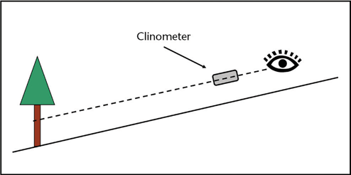
Percent slope
You can measure the percent slope of the ground in your stand using a clinometer. Holding the clinometer parallel to the slope, look either uphill or downhill at an object that is approximately the same height above the ground as your eye, such as a spot on the trunk of a tree (Figure 8-1). Visually line up the marker in the clinometer with this object and read the value on the percent slope scale of the clinometer. The slope will likely be variable throughout your stand, so try to measure the slope in an area that is most representative of the slope of the stand or measure in several locations and compute an average.
Aspect
If your stand is on a slope, the aspect is the direction the slope faces (can be given as an azimuth, 0–360 degrees). Here are some common aspects:
- 0° – Flat
- 45° – Northeast
- 90° – East
- 135° – Southeast
- 180° – South
- 225° – Southwest
- 270° – West
- 315° – Northwest
- 360° – North
You can estimate aspect based on your stand map or by using a hand compass in the field. As with slope, the aspect will likely be variable throughout your stand, so pick an aspect that is most representative of the stand.
Elevation
If you do not know the approximate elevation of your property, you may be able to determine it using an online mapping tool or a GPS device.
Stand age
If you know how old the stand is, either from your records or from measuring the total age of dominant trees with an increment borer (Chapter 6), enter it on your stand data form.
On your own
For each stand on your property, collect and record stand-level data, including stand name, acreage, inventory year, site index for relevant species, slope, aspect, elevation, and age where available. Record the data on your stand data recording sheet.
Glossary
- Acre. A unit of land area measurement used in the United States. An acre is 43,560 square feet, which is equivalent to an area 1 chain wide by 10 chains (1 furlong) long (or a square with sides equal to 208.71 feet). There are 640 acres in a square mile.
- Acreage measuring grid. A grid or series of evenly spaced dots that are often printed on clear plastic and used to measure area on a map.
- Azimuth. A direction expressed in the degrees of a circle that starts with north at 0° and proceeds clockwise to east (90°), south (180°), west (270°), and back to north (360°). Also refers to a style of compass in which directions are expressed as azimuths (as contrasted with a quadrant-style compass).
- Basal area. The cross-sectional area of a tree trunk at breast height (calculated under the assumption that the cross section is roughly circular). The combined basal area of all trees in a stand on a per-acre basis is a function of both the number and size of trees. It is a measure of competition and is used to help determine whether a stand should be thinned to meet a particular management objective.
- Basal area factor (BAF). A calibration factor for prisms or keyhole angle gauges that relates each “in” tree in a variable plot to a total amount of basal area per acre (e.g., a BAF of 30 means each “in” tree represents 30 sq ft of basal area per acre).
- Base age. The age on which a site index is based, usually 50 or 100 years. For example, a site index with a base age of 50 tells how tall dominant trees can be expected to be at age 50.
- Borderline tree. A tree whose center falls directly on the plot boundary of a fixed-area plot or that appears to be right on the boundary between in and out of a variable plot.
- Breast height. 4.5 feet (54 inches; 1.37 m) above the ground on the uphill side of the tree. This is the standard location for measuring tree diameter, basal area, and age.
- Breast height age. The age of a tree measured 4.5 feet above the ground on the uphill side of the tree. Breast height age is not the total age of the tree, because it doesn’t include the years it took the tree to reach breast height.
- Chain. A length of 66 feet (20.1 m). There are 80 chains in a mile and 10 square chains in an acre.
- Circular plot. A sample plot that is in the shape of a circle (rather than a square or rectangle).
- Circumference. The length of the outer edge (perimeter) of a circle.
- Clinometer. An instrument for determining tree height by measuring vertical angles between your eye and the top and bottom of a tree.
- Competition. The fight for resources (light, water, nutrients) among neighboring trees.
- Conifers. Cone-bearing trees. Examples include pine, fir, hemlock, spruce, cedar, and larch.
- Declination. The difference between geographic (true) north and magnetic north. Compasses must be adjusted for declination so that they point to geographic north.
- Diameter. The width of a circle or cylinder.
- Diameter at breast height (DBH). The width of a tree trunk measured 4.5 feet above the ground on the uphill side of the tree.
- Diameter tape. A special measuring tape calibrated so that when wrapped around the tree’s circumference, it reads diameter units (circumference divided by π).
- Dominant tree. A tree with the highest crown position above the majority of surrounding trees.
- Expansion factor. Converts values (number, basal area, volume, etc.) from an individual tree basis to a per-acre basis. For example, one tree with an expansion factor of 10 represents 1 × 10 = 10 trees per acre.
- Extrapolate. To use known information to make inferences about unknown conditions (e.g., using sample plot data to infer stand-wide values).
- Fixed area plot. A sample plot that has a defined size (e.g., 1/10 acre).
- Furlong. A length of 10 chains, or 660 feet (201.2 m).
- Geographic north. The “true” north (the location of the North Pole). Magnetic north, located in the Canadian Arctic, shifts over time. Declination is the difference between magnetic and geographic north. Compasses should be adjusted for declination so that they will point to geographic north.
- Glass wedge prism. A piece of specially cut glass that deflects light and shifts the image of a tree when viewed through it. Used to determine “in” trees in variable-radius plots.
- Hardwoods. Broadleaf (usually deciduous) trees such as maple, oak, alder, ash, cottonwood, cherry, and birch.
- Increment borer. A hollow drill-like tool used to extract an increment core so that annual rings can be counted to determine age.
- Increment core. The thin piece of wood extracted from a tree using an increment borer.
- Keyhole angle gauge. A tool with variously sized openings used to determine “in” trees in a variable plot and to measure basal area/acre.
- Landscape Management System (LMS). A forest inventory computer program used to analyze inventory data, project forest growth, and evaluate management alternatives.
- Live crown ratio. The proportion of a tree’s total height that contains live foliage.
- Logger’s tape. A retractable tape with distances on one side and diameter measurements (via diameter tape scale) on the other.
- Magnetic north. The direction a compass points. Different from geographic north and changes over time. Compasses must be adjusted for declination.
- Overstory. The trees in a stand that form the upper canopy.
- Pacing. Counting steps to measure distance. Every other step is counted as one pace.
- Percent slope. The change in vertical elevation per 100 feet of horizontal distance.
- Plot boundary. The outer edge of a fixed-area plot. Trees falling inside are considered “in.”
- Plot radius. The distance between plot center and the plot boundary.
- Plot sampling. A method of sampling a stand by measuring small representative areas instead of every tree.
- Quadrant. One-quarter of a circle (90° arc). Also refers to a compass style that measures directions by quadrant.
- Reference point. An identifiable location used as the starting point for a sample plot grid.
- Sample bias. When plots do not accurately represent the larger area.
- Sample plot. A small area used to represent a stand. Only trees in the sample plot are measured.
- Scale. A map measurement conversion (e.g., 1 inch = 1,000 feet).
- Site index. A measure of productivity based on the expected height of dominant trees at a standard base age (usually 50 or 100 years).
- Snag. A standing dead tree.
- Species composition. The mixture and relative proportions of tree species in a stand.
- Stand. A distinct, recognizable management unit consisting of a contiguous area that is relatively uniform in species composition, age, structure, etc.
- Systematic sampling. A sampling procedure in which sample plots are selected based on objective, pre-determined criteria (such as on a grid) rather than at random or convenience (e.g., locating plots near a road).
- Taper. The progression of the diameter (width) of a tree from wide at the base to a narrow point at the top, giving the stem of the tree a cone shape.
- Tarif number. A number used to characterize tree taper and volume based on both the diameter and height of the tree. An average tarif number may be computed for a whole stand.
- Tarif access table. A table listing tarif numbers for a given species by DBH and height (see Appendix A).
- Thinning. The removal of some of the trees in a stand, making more resources available for the remaining trees. Thinning is done to increase the growth, vigor, and/or quality of the remaining trees, improve forest health, reduce fire risk, stimulate understory growth, generate wood products, and other reasons.
- Total age. The complete age of a tree from when it first started growing, not just from the point at which it reached breast height. Total age is usually about 4–5 years longer than breast height age.
- Trees per acre (TPA). A basic measure of how dense a stand is, expressed as the average number of trees that would be found on one acre of land.
- Uniformity. Similarity in a group of trees (e.g., same species, similar size, even spacing).
- Variable plot. Sample plots that do not have a specifically defined plot radius or plot boundary. A glass wedge prism or keyhole angle gauge is used to determine whether a tree is “in” or “out” rather than the tree’s location within a defined boundary. The larger a tree is or the closer it is to plot center, the greater the likelihood of it being “in” the plot.
- Volume table. A table listing the approximate volume of wood in a tree based on its diameter and usually some other variable such as height or tarif number.
- Woodland stick. Also called a Biltmore stick or a cruiser stick. This inexpensive tool resembles a yardstick and is used to measure tree heights and diameters quickly and easily (though not as accurately as with a clinometer or diameter tape).